Scores from the Kendama World Cup 2025

My friend recently showed me the final scores from the Kendama World Cup 2025:

World Cup 2025 Final Scores

I decided to plot out the distribution of scores.

import pandas as pd
import matplotlib.pyplot as plt

scores = [
    2043, 1622, 1457, 1448, 1403, 1395, 1371, 1347, 1285, 1277,
    1206, 1205, 1159, 1113, 1063, 1062, 1008, 1000, 1000, 956,
    948, 939, 938, 924, 917, 911, 910, 885, 872, 869, 820, 797,
    772, 729, 703, 666, 665, 662, 578, 536, 485, 472, 452, 340,
    306, 273, 82
]

df = pd.DataFrame({'score': scores})

plt.figure(figsize=(10,6))
plt.hist(df['score'], bins=10, edgecolor='black')
plt.xlabel('Score')
plt.ylabel('Frequency')
plt.title('Kendama World Cup 2025 Scores Histogram')
plt.show()

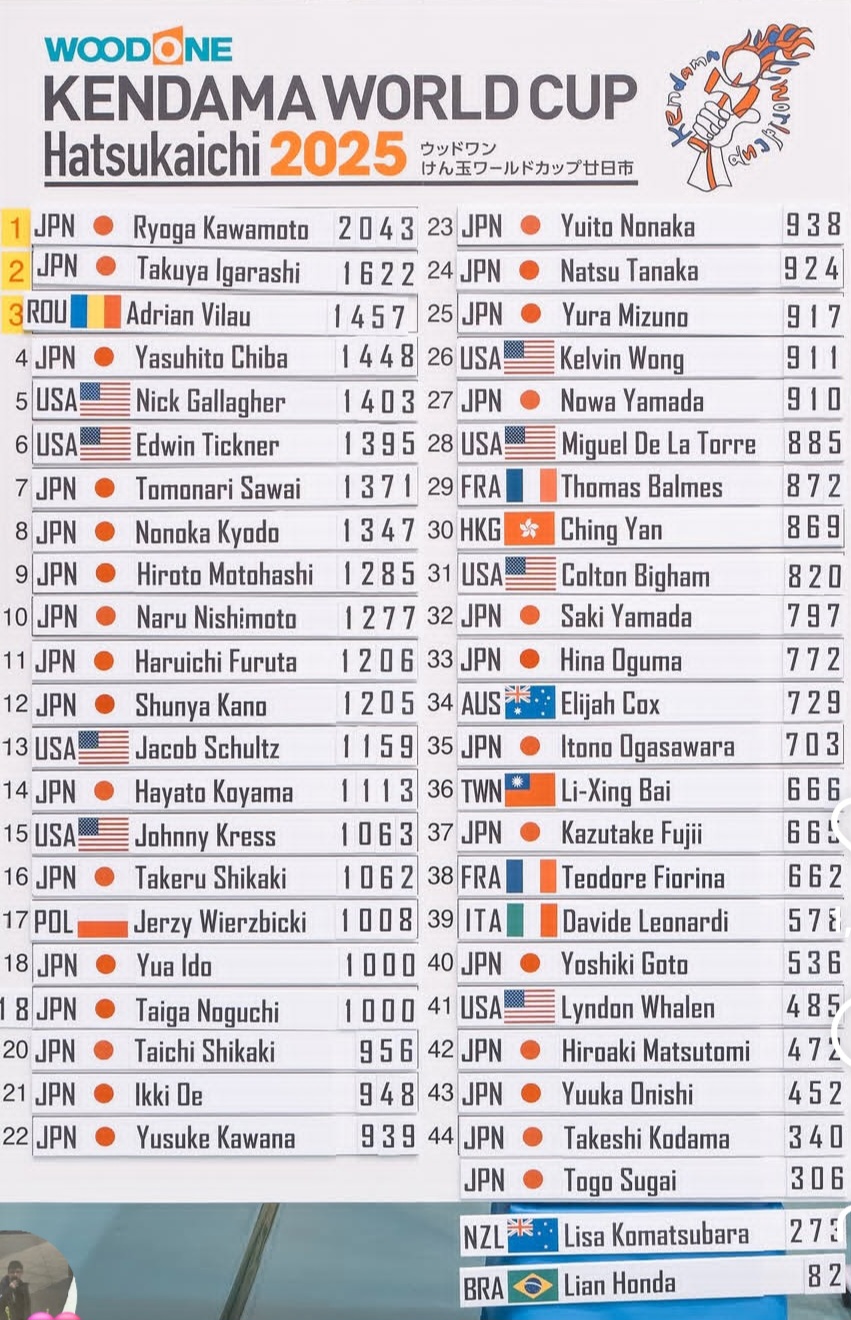
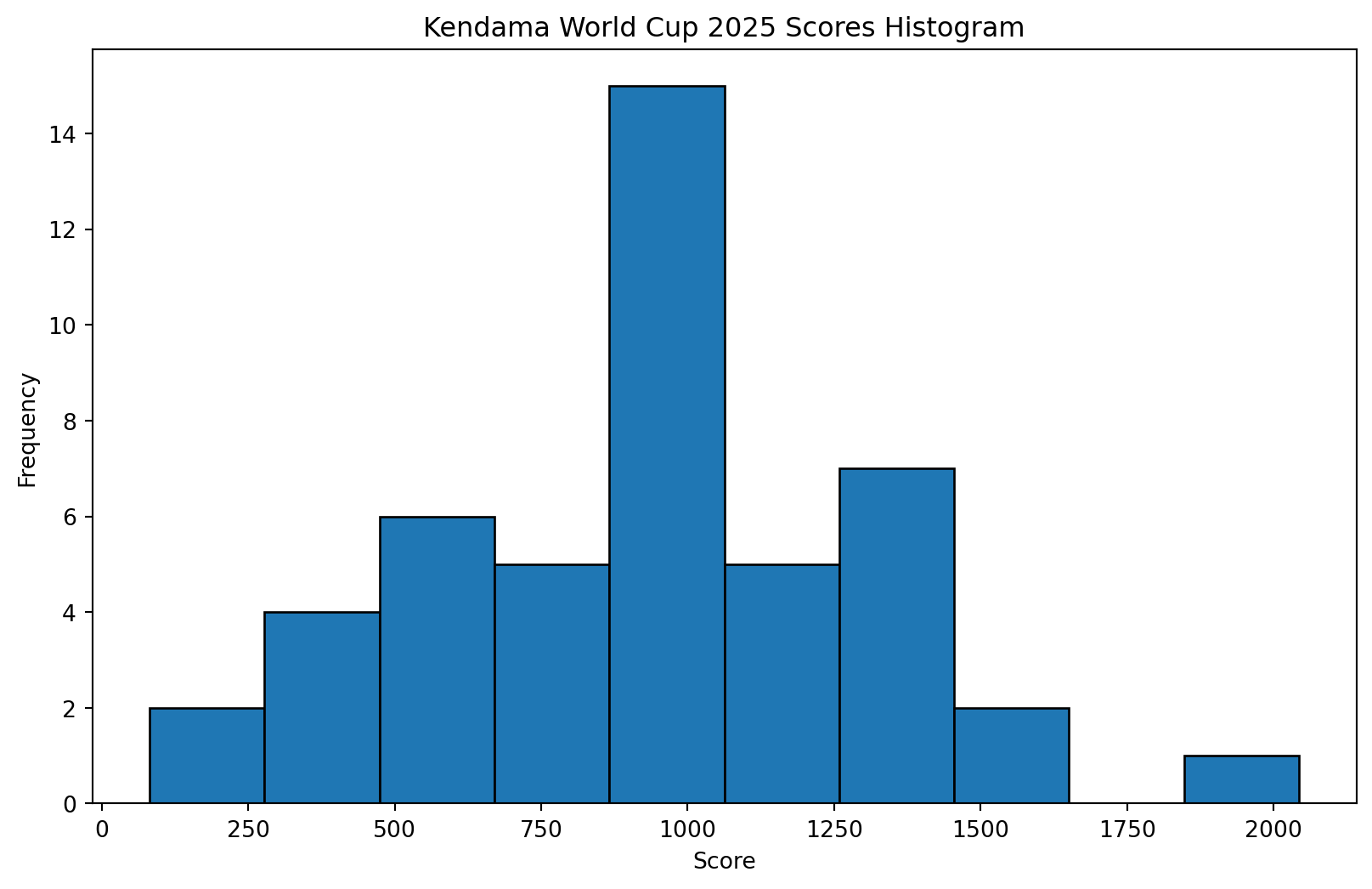
To my surprise the distribution looks bell-shaped, with a very obvious peak at 1000! So while the table form is useful to look up player names and scores, the histogram is even more insightful. I did not expect scores from a competition to also be distributed with such a familar shape. What steps can I take next to see if the scores are normally distributed? Can I apply Central Limit Theorem to make any inferences?